A physical layer full of opportunities
Exploring the story of the physical layer in the OSI model of computer networks.
Now we come to the first layer of the OSI model of computer networks: the physical layer. Here I will use the professor’s slides as a framework to briefly discuss the story of what happens in the physical layer, mainly focusing on the transformation process between digital and analog signals, which is a battle between discrete and continuous. The reason why it is full of opportunities is that there are hidden spells between discrete and continuous waiting for us to acquire.
Signals and Information
To understand all the interesting things that happen in the physical layer (mainly mathematical stories, of course), there is still some preparatory work to be done. Let’s take a look at what the physical layer actually does.
The physical layer uses the transmission medium to establish, manage and release the physical link for both ends of the communication to achieve transparent transmission of the bit stream and to ensure that the bit stream is correctly transmitted to the opposite end. The physical layer carries the bitstream in bits. I know I’ve made this clear, but you may still be walking on clouds and not know what’s going on. So let me use a real life example to help you understand better.
For example, if you are talking to a friend, the content of your speech needs to be programmed by your brain, and then the content of what you are going to say is sent to your mouth, and your mouth makes the other person hear what you are saying by making a sound. And you don’t have to think about how the sound waves will be transmitted to the other person’s ears when you speak, and you can’t see how the sound waves are transmitted to the other person’s ears. Here the sound waves can be understood as a ‘bit stream’, and your mouth is providing the ‘physical layer’.
The mouth is responsible for starting the conversation (establishing the link), judging the start and end of the conversation (managing the link), and ending the conversation (releasing the link). And the mouth also does not have to think about how the sound waves reach the other person’s ears, so the sound waves are transparent to the mouth. Transparency' in the network = low management cost.
We know that binary codes can be conveyed through changes in the strength of a signal, and these codes are recognized as different symbols through which a variety of information can be conveyed. In information theory we can actually quantify information by introducing the concept of entropy (entropy) in physics, and the amount of information contained in the received message is also called information entropy. In fact, in 1948 Shannon did just that, by introducing the entropy of thermodynamics into informatics. We can then define information in this way.
Information, on the one hand, can be understood as the uncertainty of being able to predict changes in the signal. Thus the information content of x in an alphabet X depends on the probability of occurrence of that x at the time of observation of the information carrying signal, and is then defined as $$ I(x)=-\log_{2}{p(x)} $$ The unit is bit.
The information entropy can then be given by finding the expectation: $$ H(X)=\sum_{x\in X} p(x)I(x) = - \sum_{x\in X}p(x)\log_{2}{p(x)} $$
Signaldarstellung
There are two types of signals transmitted in the physical layer transmission medium, analog signals, and digital signals, examples of which are given in the following figure.
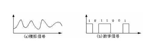
Analog signal and digital signal
Since the computer can only recognize digital signals, but to propagate in the WAN but in the form of analog signals (the case of fiber optics is different again, this is an afterthought), we will set up a modem to convert the digital signals into analog signals and the reverse process.
And next we will discuss the details of these two processes.
Mathematical Basics
At the beginning, it is said that the story of the physical layer is a contest between discrete and continuous. Although there is only a contest between the two relative concepts of discrete and continuous, the two can be converted into each other using the right method, which is the magical mathematical spell we are going to explain in this part.
Of course if you have enough enlightenment you can comprehend the two epic level spells again.
Fourier series
In mathematics, the Fourier series decomposes any periodic function or periodic signal into a collection of (possibly infinite elements) simple oscillatory functions, i.e., sine and cosine functions, and is also the core of the sampling theorem we will talk about later.
I give here directly the definition above the professorslides.
Ein periodisches Signal s(t) lässt sich als Summe gewichteter Sinus- und Kosinus-Schwingungen darstellen. Die so entstehende Reihenentwicklung von s(t) bezeichnet man als Fourierreihe:
$$ s(t)=\frac{a_0}{2} + \sum_{k=1}^{\infty} {a_k\cos{k{\omega}t} + b_k\sin{k{\omega}t}} $$
Here the $a_0$ is the offset relative to the y-axis, while $a_k$ and $b_k$The two coefficients can be defined by:
$$ a_k = \frac{2}{T}\int_0^T {s(t)\cos{k{\omega}t}} {\rm d}t $$
$$ b_k = \frac{2}{T}\int_0^T {s(t)\sin{k{\omega}t}} {\rm d}t $$
Fourier transform
The Fourier transform is a linear integral transform used to transform a signal between the space-time and frequency domains. In fact, to borrow from Wikipedia, the Fourier transform is like a chemical analysis that determines the basic components of a substance; a signal comes from nature and can be analyzed to determine its basic components.
Die Fourier-Transformierte einer stetigen, integrierbaren Funktion s(t) ist gegeben als $$ s(t) \longrightarrow S(f) = \frac{1}{\sqrt{2\pi}}\int_{t=-\infty}^{\infty} {s(t)(\cos{2\pi ft}-i\sin{2\pi ft})} {\rm d}t $$ Of which $i=\sqrt{-1}$ , Of course, it can also be written in exponential form here, so I won’t go over it again。
Sampling, Reconstruction and Quantification
With the previous mathematical foundation, we can begin to learn about the signal processing process of sampling (Abtastung), reconstruction (Rekonstruktion), and quantization (Quantisierung), which leads to the exciting transformation between discrete and continuous. More specifically, the combination of sampling (time domain discrete) and quantization (value domain discrete) converts analog signals into digital signals, while reconstruction can be considered the inverse of sampling. The famous “Nyquist-Shannon sampling theorem”, is a basic bridge between continuous and discrete signals, and is actually more like a constraint for conversion. We will talk about this in more detail later.
Abtastung
Let’s start here by looking at what Wikipedia has to say:
In the field of signal processing, sampling is the process of converting a signal from an analog signal in the continuous time domain to a discrete signal in the discrete time domain, implemented with a sampler. Usually sampling is performed jointly with quantization, and the analog signal is first sampled by a sampler at a certain time interval to obtain a temporally discrete signal, which is then also numerically discretized by an analog-to-digital converter (ADC) to obtain a digital signal that is both numerically and temporally discrete.
The signal obtained by sampling is a discrete form of a continuous signal (for example, a real-life signal indicating pressure or speed). Continuous signals are typically sampled by an analog-to-digital converter (ADC) at regular intervals, when the value of the continuous signal at that point in time is represented as a discrete, or quantized, value.
The discrete form of the signal thus obtained often introduces some errors into the data. The errors come from two main sources, the sampling frequency related to the spectrum of the continuous analog signal, and the word length used for quantization. The sampling frequency refers to the frequency at which a continuous signal is sampled. It represents the accuracy of the discrete signal in and time and spatial domains. The word length (number of bits) is used to represent the value of the discrete signal, and it reflects the accuracy of the signal’s magnitude.
Let’s see what the professor’s slide says:
Das Signal s(t) wird mittels des Einheitsimpulses (Dirac-Impulses) $\sigma[t]$ in äquidistanten Abständen $T_a$ (Abtastintervall) für n $\in$ Z abgetastet: $$ \hat{x}=s(t) \sum_{n=-\infty}^{\infty}\sigma[t-nT_a]= \begin{cases} 1, & t=nT_a \newline 0, & sonst\ \end{cases} $$ Da $\hat{s}(t)$ nur zu den Zeitpunkten nTa für ganzzahlige n von Null verschieden ist, vereinbaren wir die Schreibweise $\hat{s}[n]$ für zeitdiskrete aber wertkontinuierliche Signale.
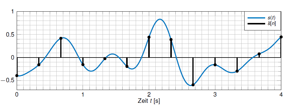
Zeitkontinuierliches Signal und Abtastwerte
Reconstruction
In this process the digital signal is converted to an analog signal as if the sampling process were reversed, called demodulation, and on an ideal system the output is instantaneously changed to that intensity every time a new data is read after a fixed time of sampling. After such instantaneous conversion, the discrete signal will essentially have a large amount of high frequency energy and harmonics associated with the multiple of the sampling rate. To destroy these harmonics and make the signal smooth, the signal must pass through some analog filter that suppresses any energy that is outside the expected frequency domain.
The multiplication in the time domain corresponds to the convolution in the frequency domain. $$ s(t) \delta [t -nT] \rightarrow \frac{1}{T}S(f)*\delta[f - n/T] $$

Reconstruction
Shannon’s Theorem
Shannon’s theorem gives the relationship between the upper limit of the transmission rate of channel communication and the signal-to-noise ratio and bandwidth.
Abtasttheorem von Shannon und Nyquist Ein auf |f | $\leq$ B bandbegrenztes Signal s(t) ist >vollständig durch äquidistante Abtastwerte ˆ s[n] beschrieben, sofern diese nicht weiter als $T_a \leq$1/2B auseinander liegen. Die Abtastfrequenz, welche eine vollständige Signalrekonstruktion >erlaubt, ist folglich durch:
$$ f_a \geq 2B $$ nach unten beschränkt.
Quantification
………
Transmission channel
For noiseless, M channels, we will have $M = 2^N$ kinds of distinguishable symbols, how does the achievable data rate vary?
Let us first recall the entropy. Assume that the source transmits all signals with the same probability such that the entropy (and hence the average information) of the source is maximum.
For a transmission rate over a channel of width B, we obtain the maximum transmission rate of
Harleys Gesetz $C_H = 2B \log_{2}(M) bit$
There is also a new definition: Signal Power (Signallesitung) The expected value of the square of the signal amplitude corresponds to the square of the signal power. The amplitude of the variance (dispersion) signal corresponds to the signal power without the DC component and represents the power of the information-carrying volume signal.
……